The first cat-circuit regression
Ten exact comparisons passed. The recorded activity, recovered dependencies and failed attempts behind our first successful small-model run.
We have run the authors' small cat visual-cortex configuration and matched its saved reference outputs. All ten original comparisons passed: six for spike times and four for membrane voltage. None were skipped, and we kept the original exact-equality criterion.
This establishes a working software regression for one small configuration. The reference is another simulation supplied by the authors. It is not an independent animal recording, and this result does not establish full-paper reproduction or a functioning neural controller.
The successful run is 20261007T235207Z-8aa25b84. The server recorded its start on 7 October at 23:52 UTC, which is 8 October in our journal's Europe/Vienna timezone. Its machine-readable result, original JUnit report and complete test log are public.
What the simulation produced
The figure below compares one recorded neuron's membrane voltage and one cortical population's spike raster with the authors' saved data. Both come from the actual retained arrays. The overlapping voltage traces and matching rasters illustrate the result; the numeric tests, rather than visual similarity, determine the pass.
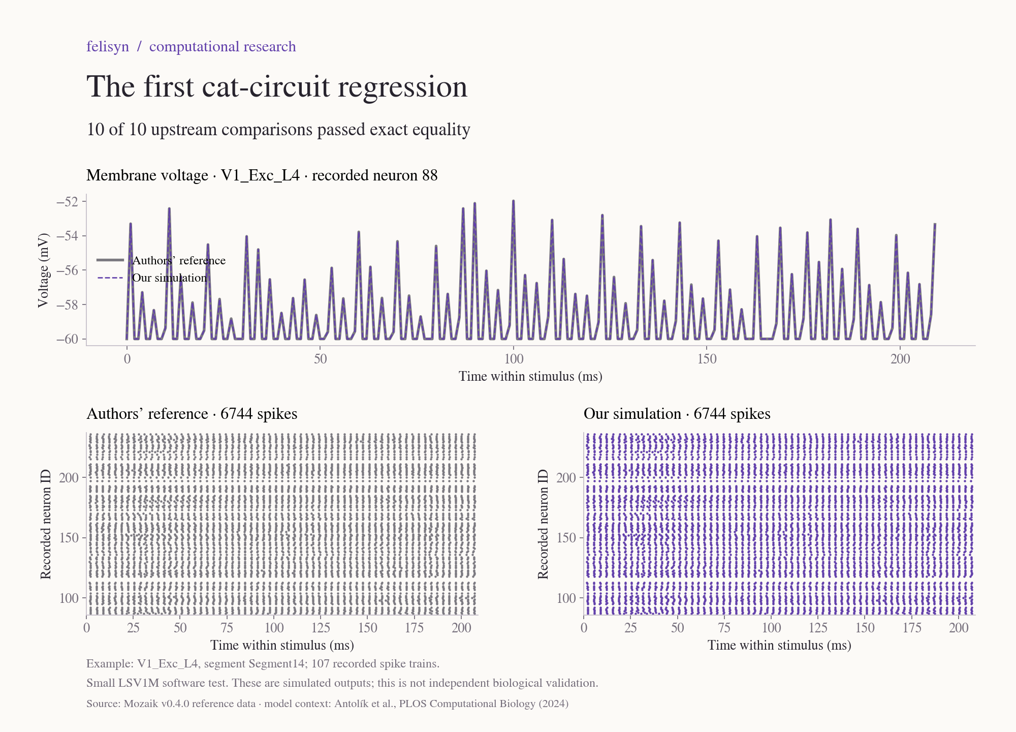
The example follows a fixed selection rule: the first segment in the upstream loader's ordering for V1_Exc_L4, then the lowest recorded voltage-neuron ID. That loader orders segment identifiers lexicographically, so this is not the first stimulus chronologically. The complete comparison covers three non-terminal-blank stimulus segments per population.
| Population | Spike neurons | Spike times | Voltage neurons |
|---|---|---|---|
| X_ON | 5 | 119 | — |
| X_OFF | 5 | 173 | — |
| V1_Exc_L4 | 107 | 16,911 | 10 |
| V1_Inh_L4 | 19 | 6,215 | 4 |
| V1_Exc_L2/3 | 116 | 18,301 | 10 |
| V1_Inh_L2/3 | 24 | 12,078 | 6 |
These are recorded subsets, not the size of a cat brain or even the complete simulated network. Across the compared segments there are 53,797 spike times and 15,750 cortical voltage samples. Counts do not represent independent biological observations. The four voltage tests allow up to 25 recorded neurons per population; this configuration records fewer. The terminal EndOfSimulationBlank segments are excluded by the original test.
Our supplemental diagnostics match segment identifiers, stimulus annotations, neuron identities, signal start/stop times and values. They agree exactly too. This supplements the upstream tests, which flatten recordings within each population; it does not replace their acceptance rule.
Recovering a compatible environment
The passing run used Ubuntu 24.04.5 LTS x86_64, Python 3.9.20, GCC 11.5.0, NEST 3.4, the custom step-current extension and a recovered custom PyNN revision reporting version 0.11.0. The host has four virtual CPUs and approximately 8 GiB of memory. The environment record and resolved source identities preserve the details.
One earlier choice needed correction. In the protocol note, we selected a PyNN candidate by filtering the current custom branch's history to commits before the framework release. That did not recover the historical custom implementation we needed. A later rebase had changed the branch history available through that route.
We found the maintainers' backup/PyNNStepCurrentModule-before-rebase-20260622-105140 branch and recovered commit 981853dd567cefb3e337accc5c13e1c8c99385ad, dated 7 June 2023. It retains the recording interface expected by this framework. After installing it, the original comparison passed. The saved remote-branch inventory and commit record document the recovery.
This is an observed compatible reconstruction. We still cannot claim that it is the exact environment originally used to generate the reference files. The original candidate remains in the earlier protocol record; the successful environment is recorded separately.
The failures belong in the record
There were installation failures before the first model attempt. Neo 0.12.0 required quantities 0.14.1 or newer, which conflicted with our initial 0.13.0 pin. mpi4py 3.1.6 also failed with a newer isolated build toolchain; pinned build tools and installation without build isolation resolved it. NEST's detached Git checkout generated an invalid Python package version, so we built a Git-free export of the same pinned source, allowing it to identify itself as version 3.4.
Then came three preserved execution attempts:
- Missing runtime dependency. The first attempt stopped during setup because Sphinx was absent. We installed Sphinx 7.4.7 and recorded the resulting package changes, including requests 2.32.5. All ten cases had setup errors; no completed neural comparison occurred.
- Incompatible recording interface. The second attempt constructed the model and began simulation, then failed while saving recordings with
KeyError: source_id. All ten cases again had setup errors. This was a dependency failure, not a measured spike or voltage mismatch. - Recovered custom PyNN. The third attempt completed simulation, saved the datastore and passed all ten comparisons. We changed the dependency implementation, leaving the model parameters, reference outputs and equality criterion intact.
The downloadable evidence package preserves all three attempts and the installation logs. The file manifest records SHA-256 hashes so the published files can be checked. Warnings remain in the logs rather than being removed from the record.
What it cost to run this test
GNU time measured 135.83 seconds for the pytest command and a maximum resident set size of 462,724 KiB, about 451.9 MiB. The original resource report is retained.
That wall time includes test setup, model execution, saving and comparison. It excludes environment installation and is not pure simulator time. The memory statistic is the command's reported maximum RSS, not whole-server peak memory. We have one successful run, so we have no repeat-run variability estimate. These measurements cannot size the full published network.
The reproduction notes include the existing-host command and a consolidated fresh-host recipe. The latter uses the recovered source pins and observed package constraints, but has not yet been tested from start to finish on a second clean machine. We retain that distinction rather than calling the environment fully portable.
The next scientific test
The small configuration was supplied for software testing. Its high firing rates and tiny scale should not be presented as validated cat physiology. Our next target remains the full model's spontaneous-activity statistics in Figure 4 of Antolík et al. Before running that comparison, we need to fix the reference values, population definitions, measurement windows, metrics and tolerances, and assess the compute requirements.
That comparison will test reproduction of a published model result. Independent biological validation is a separate stage. A future controller will also need causal evidence that changing the neural dynamics changes its decoded requests under identical inputs. Today's result gives us a working starting point for those experiments.
Sources and reproducible artifacts
- Antolík et al. (2024), A comprehensive data-driven model of cat primary visual cortex.
- Mozaik v0.4.0 source, tests and saved references. The repository's CeCILL license is retained with this package. Figure 1 is a new rendering of its reference arrays and our simulated outputs, not a reused paper figure.
- Result summary, recording diagnostics and diagnostic code.
- Execution evidence package, including raw model output, all attempt logs, environment records, scripts and figure data. Manifest · Reproduction notes.