Matching the recording configuration
The archived recording grids match the general release configuration in all four cortical populations. We separate that finding from unresolved historical software details.
The recording mismatch identified in our previous note now has a clearer explanation. We recovered the archived parameter tree and compared it with both released configurations of the cat visual-cortex model. All four cortical populations use recording grids that match the general param recipe. All four differ from param_spont.
This matters because two runs can simulate similar networks and still measure different cells. Before comparing their summary statistics, we need to know how those cells were selected. The comparison gives us a better candidate for the next experiment, while leaving several historical software questions open.
What we recovered
Our reference remains Figure 4 of Antolík et al. (2024). We retrieved the selected run's parameter record, four experiment definitions and its associated recording, stimulus and result metadata from the public API used by the authors' archive. The run's creation field is dated 22 March 2024; the archive submission field is dated 31 October 2024. Those are different events.
For the release comparison, we used LSV1M v1.0 at commit 04bf11b… and the Mozaik v0.4.0 parameter loader at f5c09a0…. Loading resolves the nested parameter files and references without constructing a neural network. The evidence package contains the complete commit identities, selected source files, retained JSON and comparison scripts.
Same grid count, different cortical area
The archived layer 4 excitatory analog recorder specifies a 200 µm square with 10 µm spacing. The dedicated spontaneous recipe specifies a 2,000 µm square with 100 µm spacing. Both have 400 grid locations before nearest-neuron selection, but the latter covers 100 times the nominal area.
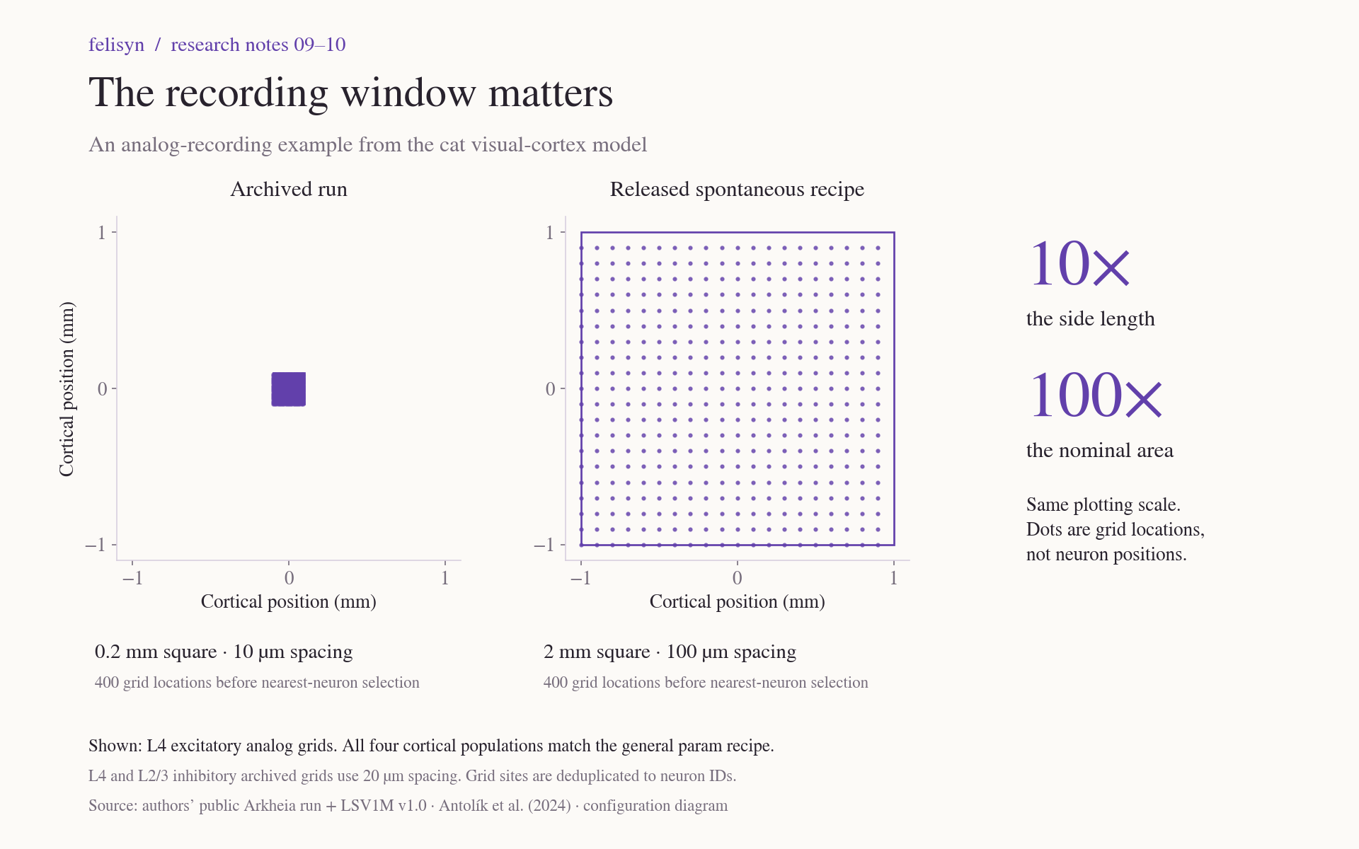
The selector finds the nearest neuron to each grid location and removes duplicate neuron IDs. Grid locations therefore cannot be reported as a count of recorded neurons. The excitatory example above also should not be generalized to inhibitory spacing: the archived inhibitory analog grids use 20 µm spacing.
| Populations | Archive and general recipe | Dedicated spontaneous recipe |
|---|---|---|
| L4 and L2/3 excitatory | 200 µm square; 10 µm spacing | 2,000 µm square; 100 µm spacing |
| L4 and L2/3 inhibitory | 200 µm square; 20 µm spacing | 2,000 µm square; 100 µm spacing |
The additional spike recorders also match the general recipe. Archived excitatory populations have extra 600 µm and 2,000 µm spike grids; inhibitory populations have an extra 600 µm grid. The dedicated spontaneous recipe instead gives each population a 3,000 µm spike grid. The exact spacings, variables and offsets are retained in the JSON comparison.
What else differs
Across the complete resolved parameter tree, the script reports 25 structural difference records against the general recipe and 47 against the dedicated spontaneous recipe. These counts describe the comparison's output structure; they are not counts of independently changed biological parameters.
Twelve differences are explicit self_connections: true fields present in the release and absent from the archive. Absence does not mean false: the effect depends on the original framework's defaults. Four differences add empty artificial-stimulator dictionaries. Six describe a changed wrapper around two afferent-delay distributions; their numeric ranges remain 1.4–2.4 ms for excitation and 0.5–1.5 ms for inhibition. The remaining three concern the results directory, stimulus storage and an added steps_get_data field.
This separates changes in representation from settings that might change the network. The full difference list preserves both values at every reported path. Determining historical self-connection behavior still requires the original framework version or equivalent evidence.
Trial labels and effective seeds
The previous note flagged archive trial 0 versus the release search script's trial 1. Source inspection narrows that concern. Mozaik's NoStimulation experiment hard-codes the stimulus's trial to 0, independently of the run-level parameter. The inspected model declares the run-level trial but does not use it to set random seeds. Those labels alone therefore do not demonstrate a change in neural dynamics.
We also traced the pinned runtime's seed handling. The parameter files contain pynn_seed: 5 and mpi_seed: 1023. Mozaik v0.4.0's controller consumes pynn_seed and, if present, mozaik_seed; it does not consume this mpi_seed field. With mozaik_seed absent, the inspected setup function supplies its default of 513. Thus the effective seeds in this pinned path are PyNN 5 and Mozaik 513. This finding applies to the inspected runtime; it does not establish which software the authors used for the archived run.
A candidate experiment, with its limits
The archive lists a 40,320 ms no-stimulation protocol, orientation tuning, natural images and size tuning. The released general experiment includes the first three, while size tuning has a separate entry point. These metadata are not a complete timestamped execution log. They do not settle the original run's full stimulus order or preceding network state.
Our reconstruction candidate is now the spontaneous entry point with param/defaults, trial 0, 16 MPI processes and one thread per process, retaining the full 40,320 ms segment. This keeps the archived recording grids. It is a declared candidate, not a certified reconstruction of every historical setting, and we have not executed the full network.
The original software revisions, historical self-connection behavior and full-precision reference arrays remain unresolved. The earlier 4.09-versus-3.56 nS source discrepancy also remains open; the individual Figure 4 means remain our declared reference. These limitations must accompany any eventual comparison.
The next question is whether our measurement code agrees with the original calculation when both receive exactly the same saved data. The following entry reports that test.
Evidence and sources
- Versioned methods and reproduction instructions, configuration summary, evidence ZIP and SHA-256 manifest.
- Retained archive run, experiment metadata and retrieval record.
- Antolík et al. (2024), LSV1M v1.0 and Mozaik v0.4.0. Original source licenses are retained.