Measuring spontaneous activity
Twenty-four published reference values, the code behind their measurement, and a recording mismatch to resolve before the full-model run.
Our next experiment asks whether we can reproduce the spontaneous activity of a published cat visual-cortex model. Before running the larger network, we need a precise account of what was measured, which neurons were sampled and how agreement will be assessed.
We have now transcribed 24 published reference means, traced their calculations through the original source and implemented measurement helpers that pass 11 analytic software tests. We also found differences between the archived run and the released recording configuration. The full-model comparison has not been run, and its final acceptance criterion remains open.
This follows our small-model regression. That earlier exact match established a working software baseline. The present step defines the next scientific comparison; it does not add a new neural result.
A reference we can inspect
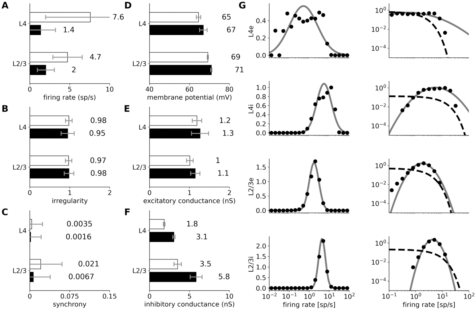
The target is Figure 4 of Antolík et al. (2024), A comprehensive data-driven model of cat primary visual cortex. It summarizes activity in the absence of patterned visual stimulation, with a uniform gray background. Four cortical populations are measured: excitatory and inhibitory cells in layer 4 and layer 2/3.
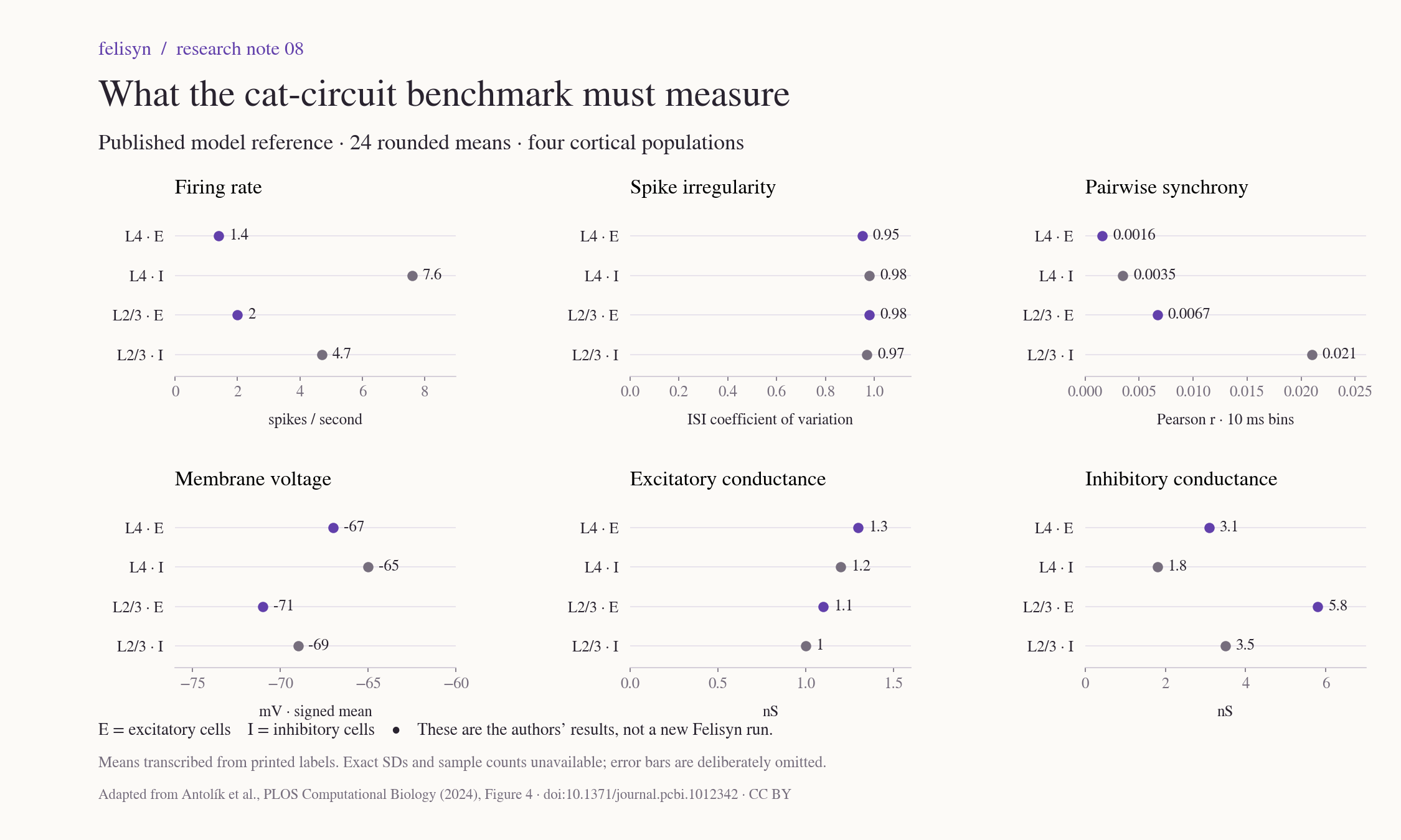
We recovered the published figure and inspected the authors' archived V1 run, dated 22 March 2024. Its displayed Figure 4 mean labels agree with the publication. The chart below redraws those labels. Every point is a published model value, not an output produced by Felisyn.
| Population | Rate, Hz | ISI CV | Correlation | Voltage, mV | Exc. conductance, nS | Inh. conductance, nS |
|---|---|---|---|---|---|---|
| L4 excitatory | 1.4 | 0.95 | 0.0016 | −67 | 1.3 | 3.1 |
| L4 inhibitory | 7.6 | 0.98 | 0.0035 | −65 | 1.2 | 1.8 |
| L2/3 excitatory | 2.0 | 0.98 | 0.0067 | −71 | 1.1 | 5.8 |
| L2/3 inhibitory | 4.7 | 0.97 | 0.021 | −69 | 1.0 | 3.5 |
These are transcriptions of printed numbers, not full-precision arrays. The source's error bars represent standard deviations across sampled neurons or pairs. We have not recovered their exact numeric values or the underlying sample counts, so we have omitted error bars from our redraw. Treating the source bars as confidence intervals or acceptable simulation-error margins would be unjustified.
Details the caption does not settle
We traced the measurements to SpontStatisticsOverview in LSV1M v1.0 and the pinned Mozaik framework. The full measurement specification records the source identities and algorithms.
The released spontaneous protocol specifies 40.32 seconds, although the paper caption says 40 seconds. We will retain the saved segment boundaries rather than silently shorten the recording. With 10 ms bins, that duration gives 4,032 bins. A uniform background is still sensory input; “spontaneous” does not mean all input is disconnected.
Firing rates include recorded silent neurons. Irregularity is the standard deviation of a neuron's interspike intervals divided by their mean. The plotting code includes a neuron in this statistic only when it has at least seven spikes. The same inclusion rule applies to pairwise correlation. Changing that rule would change which cells contribute.
Correlation is calculated from 10 ms histograms, with each pair counted once and self-pairs excluded. The framework converts undefined correlations to zero. We preserve that convention for comparison and also count the affected pairs so the substitution remains visible. Neuron IDs must be aligned before a population mask is applied.
Voltage and conductance summaries first average each neuron's signal over time, then summarize those per-neuron means. We preserve negative membrane voltages and explicitly convert conductance from microsiemens to nanosiemens. All these population SD calculations use the source's ddof=0 convention.
A recording mismatch to resolve
The archived parameters give us more than a picture. For layer 4 excitatory cells, the original run records analog signals on a 200 µm square grid with 10 µm spacing, plus additional spike recordings. That matches the release's general param configuration.
The dedicated param_spont recipe instead uses a 2,000 µm analog grid with 100 µm spacing and a 3,000 µm spike grid with 20 µm spacing. These are grid dimensions, not cell counts: the selector finds the nearest neuron to each grid point and deduplicates the result. We verified the archived comparison for layer 4 excitatory cells; the remaining populations still need the same check.
There is another subtlety. The plotting class computes a central-region mask but does not use that mask in its six summary measurements. The paper's general methods describe a different spatial selection. This does not establish that the published result is wrong. It means that running the released spontaneous recipe is not yet demonstrated to sample the same cells as Figure 4.
The archive also reports trial 0, while the released parameter-search script selects trial 1. The general experiment begins with the same 40.32-second spontaneous stimulus, which gives us a concrete route to investigate. We still need to reconcile the original run's full configuration and stimulus history before freezing an exact reproduction recipe.
Keeping conflicting source values visible
The paper's prose reports a pooled inhibitory conductance of 3.56 nS. Applying the plotting code's weights to the four rounded inhibitory-conductance labels gives 4.09 nS. The difference is larger than rounding of these labels can explain under that weighting.
We have not established the cause. Our declared reference is the set of individual Figure 4 means above; the prose value remains a separate unresolved source discrepancy. We will not switch targets after seeing which one a new run matches. The derivation and source lines are retained in the evidence package.
What we built and tested
The new metric helpers implement the single-window calculations independently. Eleven analytic tests cover silent neurons, the six-versus-seven-spike boundary, a known interval-variability result, unique pairs, undefined correlations, units and invalid input. They also check that matching a rounded printed number cannot produce an overall benchmark pass.
All eleven passed; the test log and machine-readable receipt are retained. These tests use explicitly synthetic edge cases. They verify calculation behavior, not neural physiology. Integration with the full datastore, time alignment of analog inputs and end-to-end agreement with the original analysis still need testing.
Our comparison policy is now explicit: report every metric and its signed difference, disclose sampling and configuration changes, preserve raw evidence and do not use neuron-to-neuron SD as run-to-run uncertainty. Agreement at the source's printed precision is descriptive only. We cannot honestly freeze a biological equivalence margin from this one rounded figure.
The next execution decision
The authors report 16 processes on an EPYC 7302 with 128 GB RAM and approximately 90 minutes for their spontaneous protocol. This is a report of their setup, not a measured minimum or a promise for our hardware. Our existing 8 GiB host has completed the small regression; that result does not establish capacity for the full network.
We will first finish the configuration comparison and test the datastore-to-metric path. Then we can freeze a declared run recipe and use a temporary larger CPU host for a bounded experiment. No full-model run or additional paid machine was started during this step. The specification includes a dated compute estimate for that later decision.
The long-term controller needs more than matching this figure. A later experiment must show that specified sensory inputs change the neural output and that removing or shuffling the circuit changes the behavior. Reproduction, biological validation and causal control will remain separate claims, each with its own evidence.
Evidence and sources
- Complete benchmark package, SHA-256 manifest and machine-readable protocol status.
- Antolík et al. (2024), article and Figure 4, published under CC BY.
- Archived V1 results and saved visible parameter excerpt.
- LSV1M v1.0 source and Mozaik v0.4.0 source. Original licenses accompany the retained source files.