Can the cat circuit make decisions? Calibrating and freezing the test
We built Felisyn's first decision pipeline around the cat visual-cortex model, entirely in simulation. A synthetic market signal becomes a drifting grating, the model responds, and a fixed decoder turns its spikes into buy, sell or hold requests for a simulated executor. A calibration run showed that the model passes on a grating's orientation almost exactly. Before the real test runs, we froze how we will decide whether the circuit's own dynamics change its decisions, and what happens if they do not.
Felisyn began with a question (note 1): can an identifiable neural computation become the working mechanism of an autonomous controller? We said then that an intervention would have to show whether the neural computation actually affects the controller's requests. This note sets up that test for the first time.
Everything here is simulation. The market is synthetic, the executor is a simulation with fixed limits, and no wallet, token, exchange or real order exists anywhere in the code.
The headline: the model reads out almost perfectly. On 48 calibration gratings, a fixed decoder recovered the shown orientation from the model's spikes with a median error of 1.4 degrees. So the circuit passes on its input very faithfully at this timing. The open question is whether it adds anything of its own. We have now fixed, before running it, the test that decides this and what each outcome means.
A decision pipeline around the circuit
Each decision step goes through five stages:
- A synthetic market produces a signal s between −1 and +1. Signals are independent from step to step, so any link between successive decisions can only come from the pipeline itself.
- An encoder turns the signal into a visual stimulus: a full-field drifting grating at 90° + 45°·s, at a contrast of 30 % + 70 %·|s|. It is shown for 210 ms, followed by 147 ms of grey.
- The cat visual-cortex model responds. It is never reset between steps.
- A fixed decoder reads the spikes of the model's layer 4 excitatory neurons and estimates the orientation. A strong enough estimate becomes a buy or sell request; anything else is a hold.
- A simulated executor accepts or rejects the request under a cash budget and position and order limits.
Every step is logged in four separate stages: model output, decoded request, executor decision and simulated outcome. A replay recomputes every decision from the saved spikes and must match exactly. The encoder and decoder are engineering choices with no biological or financial meaning, and we say so in every result.
A smaller copy of the published model
The full model needs about 15 hours for 40 seconds of activity on our server (note 15). That is too slow for hundreds of decisions. Mozaik's small test configuration was no alternative: every cortical neuron in it fires at about its maximum rate, 300 spikes per second for the excitatory neurons, even without a stimulus. So we use a 2 mm reduction of the published model, with the published files unchanged and three command-line settings.
In 5 seconds of spontaneous activity, the reduction is asynchronous and irregular, as the full model is. It fires somewhat faster (2.0 to 10.9 Hz against 1.4 to 7.6 Hz across the four cortical populations), its neurons are 3 to 6 times more correlated, and neurons near the edge of the smaller sheet fire more. Every result from it carries the label "2 mm reduction".
Calibration: can we read the circuit?
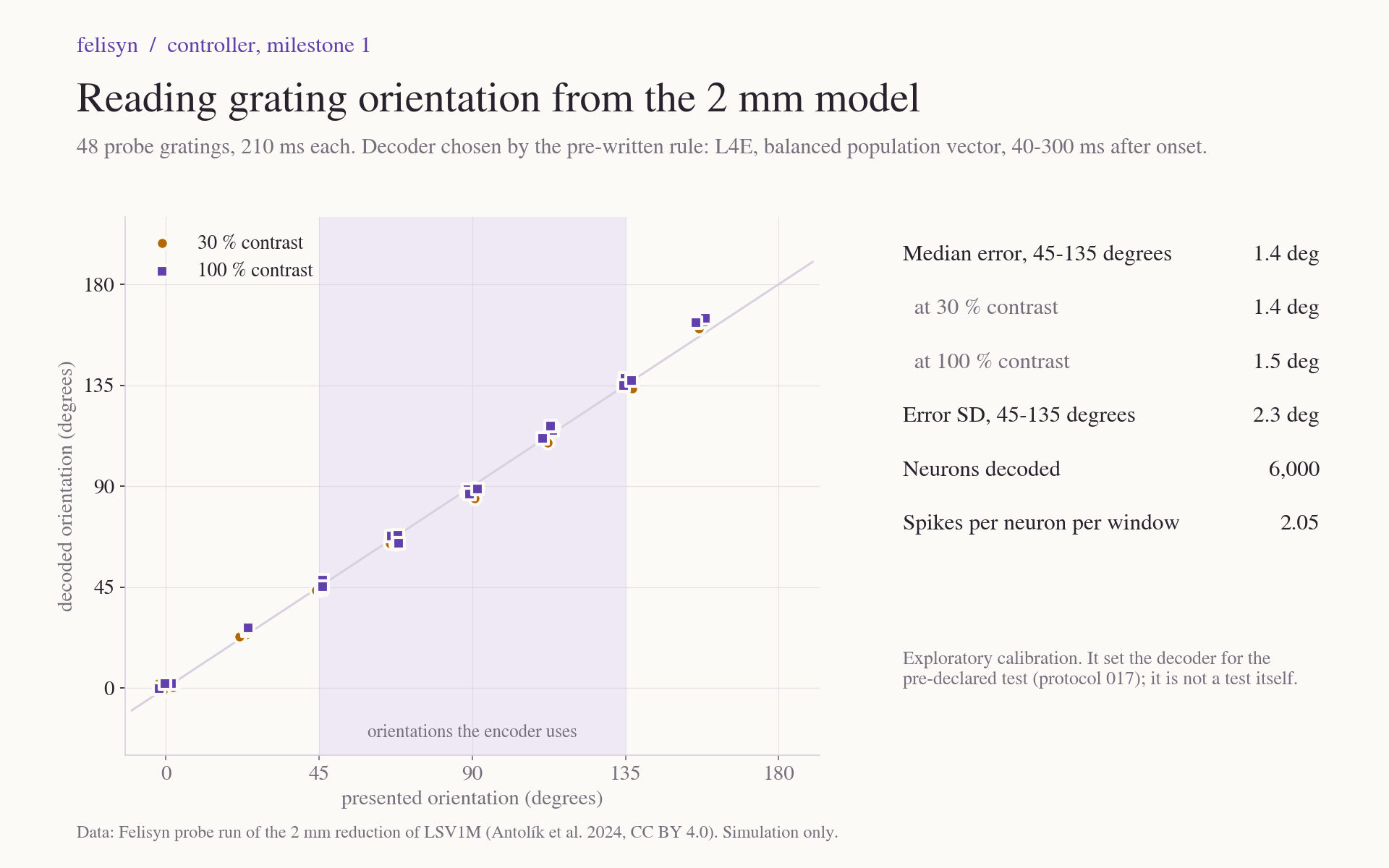
The calibration run showed 8 orientations at 2 contrasts (30 % and 100 %), 3 times each, in shuffled order, with the same timing as the test. Before its results existed, we wrote down how the decoder would be chosen from 36 candidates: 3 layer choices, 4 time windows and 3 ways of weighting the neurons. The rule takes the lowest median error over the orientations the encoder uses, and prefers the simpler variant when two are within 1 degree of each other.
The rule chose the 6,000 layer 4 excitatory neurons, counted 40 to 300 ms after each grating's onset. The weighting is "balanced", so a response that is equal across neurons adds nothing. Over 45 to 135 degrees its median error is 1.45 degrees, its standard deviation 2.3 degrees, and its largest error 5.6 degrees. Low contrast hardly matters (1.4 against 1.5 degrees). Layer 2/3 alone decodes less precisely, with a best median error of 3.3 degrees.
The run took 2 hours 15 minutes. The largest part, 52 minutes, went into computing the retina's and LGN's response frame by frame before the gratings were simulated, about 1.2 seconds per 7 ms frame. Simulating the 17 seconds of activity took 37 minutes. These costs set how long the test can be: about 110 seconds of computing per decision.
The test, declared before it runs
Protocol 017 fixes the test before any of its runs.
Three model runs, on one sequence of 120 decisions:
- intact-A: the published parameters;
- intact-B: a second network instance, with different neuron positions and therefore different connections;
- feedforward-only: intact-A's network with every connection between cortical neurons set to zero weight. The decoded layer 4 then receives only its input from the LGN.
One main measure: carry-over. For each run we fit ŝ_t = a + b·s_t + c·s_(t−1), where ŝ_t is the decoded decision signal at step t. A relay of the current input has c = 0. A circuit whose state links one decision to the next has c ≠ 0. We call carry-over material when |c| reaches 0.10. At that size, a strong previous signal shifts the current decision signal by 40 % of the buy and sell threshold. A 95 % interval for c comes from resampling blocks of steps.
Readings, fixed in advance:
- Dynamics: both intact runs show carry-over beyond the margin, with the same sign. The circuit's dynamics carry information from one decision to the next.
- Dynamics, size unresolved: both show detectable carry-over of the same sign, but its size is not shown to reach the margin.
- No carry-over: neither shows material carry-over. At this timing, any carry-over the test detects is below the margin, and following our plan this controller design stops here.
- Inconclusive: anything else.
If the decoder fails on an intact run, no reading applies. The feedforward-only run says whether any carry-over needs the cortex's own connections.
Baselines from each run's own data:
- a relay that adds the run's own errors to the input, drawn independently;
- the run's decisions shuffled across steps;
- the noiseless rule.
The number of decisions. It came from a rule written as code and recorded with its hash before the calibration results existed. The rule takes the upper confidence bound of the decoder's calibration error and asks for an interval of c no wider than ±0.05. With the decoder this precise, the minimum of 120 decisions already gives about ±0.02.
Simulated with the calibration's own errors, the test behaves as intended:
- with no carry-over, every pair of runs read "no material carry-over";
- a carry-over of 0.10 was detected in every simulated run;
- a carry-over of 0.20 always read as material.
Two reviews before freezing
An independent reviewer checked the design and the code twice. The first review found that our baseline mishandled large errors that wrap around the orientation circle. That would have made a plain noisy relay look distorted. The baseline now works in angle space, and a test shows the problem is gone.
The reviews also brought:
- a check that the decoder works before any reading applies;
- five categories for the size of the carry-over;
- an analysis that refuses mislabelled runs, changed inputs or a failed replay;
- corrected statements about which time scales in the model can link successive steps.
The model has no slow adaptation. What can link one step to the next is synaptic depression, which recovers within 20 to 70 ms inside the cortex and 125 ms between the LGN and the cortex. The LGN's 200 ms filters and the network's own recurrent activity can too.
Two short smoke runs tested the lesion before the freeze. The first removed every connection within each cortical layer, plus the feedback from layer 2/3 to layer 4, but kept the input from layer 4 to layer 2/3. Without any inhibition, layer 2/3 then fired near its ceiling: 292 spikes per second on average for its excitatory cells, against 7.6 in the intact network. The decoded layer 4 never saw this, since its feedback was cut, but it slowed the simulation almost fourfold. The declared lesion therefore also cuts the input to layer 2/3. A second smoke run confirmed that this leaves layer 4 untouched: its neurons fired exactly the same spikes as in the first run, neuron by neuron, and the decoder read them with a median error of 4.1 degrees. That is coarser than the intact network's 1.45 degrees, but the lesioned layer still clearly decodes.
What we expect
Given how faithfully the circuit relays orientation at this timing, little or no carry-over would not surprise us. The test is built so that either outcome is clear. If there is no material carry-over, we stop this design, as the project plan requires. The next step would then be a new protocol at timings where the circuit's dynamics have more room to matter. If there is carry-over, the circuit is doing something of its own between decisions, and the next steps build on it.
Limitations
- Not the full model. These are decisions of a reduced model with an engineered encoder and decoder. They say nothing about how cats decide anything.
- One market, one timing. Decisions do not feed back into the market. A shorter grey gap could change the answer.
- One kind of history. The main measure is a linear dependence on the previous signal; other forms are reported but do not change the reading.
- No financial claim. The market is synthetic and the profit or loss is simulated.
Next step: the three runs, which started at 20:47 UTC and take about 15 hours on our server, then a results note.
Model: Antolík J, Cagnol R, Rózsa T, Monier C, Frégnac Y, Davison AP (2024), A comprehensive data-driven model of cat primary visual cortex, PLOS Computational Biology, published under CC BY 4.0. LSV1M v1.0 is under its MIT license. The 2 mm reduction, the pipeline and all runs are ours. The figure is a new plot of our own run.